Our web projects come in all sorts of shapes and sizes. The vast majority of the sites we build, however, are less than fifteen pages. Smaller sites are very easy to organize. If I need a quick refresher on where we are in the project, I can glance at the site map. When challenged with a site containing more than 40 pages, this method is far less effective. There are just too many elements for one human to remember. So, when I encountered not one, but TWO giant web projects this summer, I had to come up with a new tracking strategy. Printing off the sitemap and jotting down notes here and there was not going to cut it. It was time to finally put everything I learned in my 8th-grade computer class to work and open a spreadsheet. NOTE: If you’re more of a visual learner, feel free to skip down to the video version of this tutorial.

And by Spreadsheet, I DON’T Mean Excel 

I know, the pun-ny title threw you off. As someone who hasn’t used a PC regularly since Windows XP (forever RIP), I’m not a huge fan of working in Excel. The Microsoft Suite, at least for Macs, is clunky. The menu is broken up into tabs, as well as the traditional menu at the top. I usually spend more time looking for an action than I do actually filling out the doc. Another issue I have is the portability of the files. If I start a sheet on my desktop, that’s pretty much the only place I can access it. I could also go on about hotkeys and other nuances, but you get the point. These gripes are just a few reasons why I create all my sheets using the Google Suite. It’s free, accessible on nearly any device (especially my iPhone!) and super easy to share (and collaborate!) with others. If I know my chart is finished or ready to be archived, I simply download the file as an .XLS and save it to the Roundpeg server. Then, anyone can open it up using Excel. It’s really that simple!

Setting Up the Sheet

Once I’ve opened up a fresh doc, I immediately set up the header row. This is where I really want to stress the importance of the KISS method (Keep it Simple and Straightforward). You want to include just enough information to jog your memory, but not so much that it’s going to take you 15 minutes to decide whether or not a page is finished. I also highly recommend changing the background color, then freezing that top row. (You’ll thank me later if/when your list grows so long that you need to scroll) Every project is a little different, but here are the headers I typically include in my sheet:

• STATUS – This row will also play an important role when it comes to conditionally formatting the color-coding.
• TITLE – The title of the page.
• URL – Link to the page. 
• CONTENT – Do we have the text on the page? (yes/no)
• STYLING – Has the page been styled? (yes/no)
• IMAGES – Have the final images been placed? (yes/no)
• LINKS – Are all buttons/links set up correctly? (yes/no)
• NOTES – List anything that needs to be said, but doesn’t fit the previous categories.

The next step is to put all the data from your sitemap into your sheet. I typically start with just the titles and URLs, then go back to mark yes/no in the other columns. Once we have some data entered, it’s time for the real magic to happen.

Get more Organized with Color Coding

As a lover of color, it comes as no surprise that I am a HUGE fan of color-coding my sheets. What I don’t love, though, is how cumbersome it is to change row colors on the fly. First, you have to highlight the row. Then click the paint bucket. Then click the color. It’s a lot of clicks, which is especially annoying with a longer sheet.  A few years back, I’d had enough with the clicking. I dropped what I was doing, opened a new tab, and scoured Google for faster ways to color code my sheets. That’s when I discovered the techno-voodoo known as conditional formatting.

What is Conditional Formatting?

In short, conditional formatting is a set of rules. When programmed in, these rules adjust your sheet’s formatting based on triggers. Google has a ton of great default triggers built-in, so don’t let the term “programming” intimidate you. By default, you can generate rules based on the following factors:

• Is empty/Is not empty
• Text contains/Text does not contain
• Text starts with/Text ends with
• Text is exactly
• Date is/Date is before/Date is after
• Greater than/Greater than or equal to
• Less than/Less than or equal to
• Is equal to/Is not equal to
• Is between/Is not between

These are all great, but they only apply to individual cells. I want to make the entire row the same color. In order to do that, we’re going to be creating our own custom formula. 

Customizing your Formula

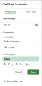
Setting up conditional formatting is easier than you may think. Once you have some data entered, right-click any cell and select “Conditional formatting” from the dropdown. (It doesn’t matter which cell you click because you’re going to set up a range anyway.) This should trigger the conditional format rules menu to slide in on the right-hand side of your window. Now we need to select our range of cells to include in the rule. You can type in the range manually, but I prefer using the little green grid icon instead. Once the “Select a data range” popup appears, click and drag over all the cells you have, or plan to have data in. Be sure to start with A2 and do NOT include your header row. Once you have your range, go ahead and click ok. We have a range, so now it’s time to create the rule. In this example, we’re going to have the row turn green if the status is set to “DONE” and red if the status reads “NEED CONTENT.” To do so, you’ll want to open the “Format Rules” dropdown and select “Custom Formula is” from the bottom of the list. This will trigger a new field titled “Value or formula.” In that field, paste in the following:

=$A2=”done”

If any of your rows statuses are set to DONE, they’ll light up green as soon as you paste in that code. If you haven’t filled in the status column yet, go ahead and test your rule by typing in the word DONE in cell A2. If it turns green, then we’re in business!

Adding Additional Rules

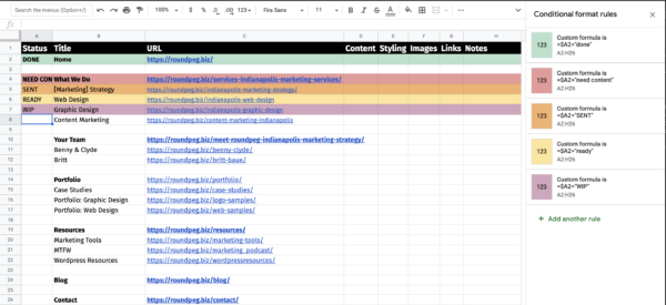
From here you can click done, but we still need to set a rule to turn rows red when the status is set to “NEED CONTENT.” To do so, go ahead and click “+ Add another rule.” This will refresh the Conditional format rules window to the last rule that’s been set. This saves us a few steps! In the “value or formula” box, either change the word “done” to “need content” or delete out the old formula and paste in this:

=$A2=”need content”

Once again, any row with “need content” in its first column will light up green. To change it to red, click the paint bucket under “Formatting style” and select red. These rows will immediately flip from green to red. You can continue down this path as many times as necessary. I like to also add rules for WIP (purple), READY (yellow), and SENT (orange).

Further Customizing your Rule Set

There are plenty of other ways to tweak this formula to your liking. You just need to understand how the formula works.  $ – tells the sheet to repeat the rule for every row below the designated cell A2 – Column, Row (In this case, the rule begins with Column A, Row 2) “Done” – The trigger. Change this to whatever word, number, or data range you wish. Just make sure to leave in the quotes!

Video Tutorial

Now it is your turn!

Build a spreadsheet and try setting a few rules. Once you get started, you may never want to go back. If you have enjoyed this tutorial, check out our new Digital Toolbox, where we are collecting all our web tips, tech tips, and other resources.